I developed this fluid dynamics simulation software in C++ and OpenGL for the CS 148 course (Introduction to Computer Graphics and Imaging) in Summer 2016. In this class, I learned about the technical underpinnings for creating computer-generated images. For my final project for this course, I reimplemented Jos Stam’s Stable Fluids algorithm for numerically stable real-time simulation of fluids for computer graphics applications (Stam 1999, Stam 2003), with the goal of approximating the convective flows that result when soap is added to milk with food coloring. I then extended my implementation with refinements for greater accuracy, including ByungMoon Kim and collaborators’ use of Back and Forth Error Compensation and Correction for Stam’s algorithm (Kim et al. 2005, Kim et al. 2007). Finally, I developed a custom OpenGL fragment shader to approximate the appearance of food coloring in milk due to subsurface scattering. Here is a recording of an interactive simulation I performed using my software:
For my efforts and accomplishments in this project, my work was recognized as “Best of Technicals” among the 47 team and individual projects presented for the Summer 2016 CS 148 course.
Motivation
My inspiration for this project came from the following music video by Michael Zoidis and Jodie Southgate:
The video consists of macro shots of food coloring and other pigments being advected (carried) by currents in a shallow pan of milk, with currents induced by soap, which acts as a surfactant. Regions with soap droplets experience convective flows, in which fluid below the surface rises up and displaces fluid on the surface. Additionally, different layers of fluid visibly slide past each other. For my project, I chose to reproduce these two essential aspects of the dye advection phenomenon captured in Zoidis and Southgate’s video.
Reimplementing Stam’s Stable Fluids Algorithm
Stam’s Stable Fluids algorithm is a grid-based fluid dynamics simulation method developed for computer graphics applications. It maintains simulation state as a set of grids of the various scalar and vector fields that describe a fluid, and it steps through time by updating the values in these grids according to the Navier-Stokes equations. Stam’s original paper focused on two-dimensional simulation with easy generalization to three dimensions, and it stored all values (including velocity) at grid cell centers; derivatives are discretized as central finite differences. For a detailed review of the mathematics and discretization of Stam’s algorithm, please refer to Section 2.1 of my mid-project milestone report. A high-level summary of the mathematics follows.
Mathematical Background
Stam’s algorithm simulates the evolution of the velocity field of an incompressible fluid and any scalar fields of quantities carried in the fluid, such as dye concentration, as governed by the following form of the Navier-Stokes equations:
$$\nabla \cdot \vec{u} = 0$$ $$\frac{\partial \vec{u}}{\partial t} = - (\vec{u} \cdot \nabla) \vec{u} - \frac{1}{\rho} \nabla p + \nu \nabla^2 \vec{u} + \vec{f}$$ $$\frac{\partial \rho}{\partial t} = - (\vec{u} \cdot \nabla) \rho + \kappa \nabla^2 \rho + s$$
The first equation enforces conservation of mass of the fluid. The second equation enforces conservation of momentum of the velocity field $\vec{u}$, with terms for the advection of velocity, generation of velocity by pressure gradients $\nabla p$ (which are projected away by Stam’s algorithm to maintain conservation of mass), dissipation of velocity with diffusion constant $\nu$, and application of external forces $\vec{f}$ to the fluid. The third equation describes the evolution of a scalar field $\rho$ whose quantities are transported by the velocity field, and this equation looks very similar to the second equation. In fact, Stam’s implementation uses the same subroutines for parts of its velocity update and its dye concentration update in each timestep.
Velocity Update
Stam presents an unconditionally stable method for updating the fluid’s velocity field, using a semi-Lagrangian calculation for velocity advection, an implicit sparse linear system for velocity dissipation (diffusion of velocity), and a vector field projection step.
Advection is done by tracing a virtual particle from each grid point of the velocity grid backwards by $d t$ in the current velocity field, estimating the velocity of the virtual particle at the resulting position by interpolation with the nearest grid points, and copying that velocity to the grid point. When $\vec{u}$ is discretized on a rectangular grid, as with Stam’s algorithm, the interpolation of the backtraced particle’s velocity can be done linearly, with bilinear interpolation in two dimensions or trilinear interpolation in three dimensions. Stam’s algorithm uses a first-order estimate of the backtraced position, by which only the current velocity at the grid point itself is used to estimate the backtraced position of the virtual particle.
Velocity dissipation is done by setting up and solving an implicit diffusion equation. This equation is in fact a sparse linear system, and Stam solves it by Gauss-Seidel iteration. However, due to discretization error in the simulation, Stam’s algorithm suffers from high numerical dissipation, which has the effect of introducing excessive artificial diffusion into the fluid; improvements to Stam’s algorithm have focused on mitigating this numerical dissipation (Kim, et al. 2005). Thus, there is no need to explicitly update the velocity field with dissipation as governed by the implicit diffusion equation.
The final step of a velocity update in Stam’s algorithm is projection of the resulting intermediate velocity field onto its divergence-free component, to maintain conservation of mass. Stam sets up a sparse linear system to solve for the gradient of the pressure field (the pure divergence component of the intermediate velocity field) by Gauss-Seidel iteration, which is subtracted out from the intermediate velocity field, resulting in the final divergence-free velocity field of the velocity update step.
Dye Concentration Update
The dye concentration scalar field is updated after the fluid velocity field. Advection is the same as with the velocity update, but the advected quantity is now the scalar field instead, so interpolation is done on the scalar field. Dye diffusion is done the same way as with velocity diffusion, and we do not explicitly calculate it for the same reasons. Finally, there is no need to remove divergence from the dye concentration field.
Reimplementation Overview
I first reimplemented Stam’s algorithm on a two-dimensional grid. For a detailed description of the software design for my reimplementation of Stam’s algorithm, including an explanation for my use of Jacobi iteration instead of Gauss-Seidel iteration for solving sparse linear systems, please refer to Section 2.2 of my mid-project milestone report. I created several classes to abstract away the scalar and vector field manipulations, and I used the Eigen linear algebra library’s Array class as my data structure to abstract away details of multidimensional array indexing and memory management. This design enabled me to easily simulate the transport of an arbitrary number of quantities or dyes. In practice, I chose to simulate three dye concentration quantities, corresponding to cyan, magenta, and yellow colors. I chose these colors to provide the subtractive model of color blending characteristic of pigment dyes, and I could add dyes of arbitrary colors by combining these quantities. While this prevented me from simulating dyes with different diffusive or color characteristics, each independent scalar field adds nontrivial computational expense, so maintaining the state of three color channel grids was a reasonable compromise.
I implemented rendering of simulation state using OpenGL’s programmable shader pipeline by sending the dye concentration grid as a texture to a fragment shader. I used and modified the structure presented in the LearnOpenGL 2D Game tutorial to render the texture on a flat rectangular canvas quad and provide user interaction, including panning, zooming, and rotation of the camera relative to the canvas. Because my dye concentrations were separate scalar grids of cyan, magenta, and yellow intensities, I sent the grids as separate single-color textures to the fragment shader, where I converted the color values to the RGB color space for color output by linearly subtracting the concentrations from 1 for the corresponding channel: $$R=1-C$$ $$G=1-M$$ $$B=1-Y$$ This also achieved the necessary effect of rendering fluid with no dye at all as white, which is the color of milk.
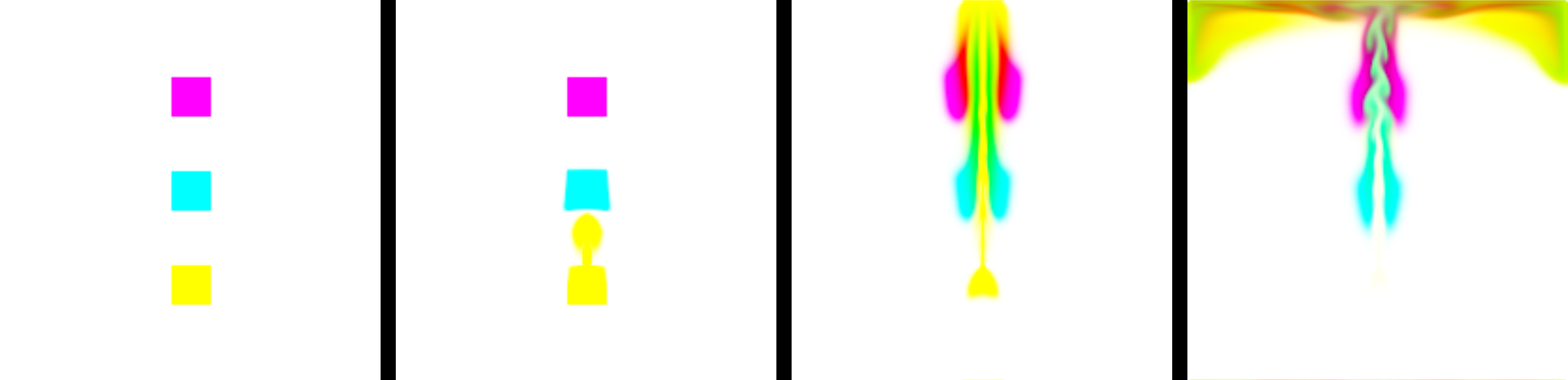
Example of a two-dimensional simulation after initial reimplementation, with four selected frames progressing in time from left to right. The third frame demonstrates subtractive color mixing, with yellow and cyan dyes mixing to produce green dye, and magenta and cyan dyes mixing to produce red dye. The fourth frame shows the rapid diffusion of dyes at the top edge due to numerical dissipation, despite the diffusion constant of the dye concentration field having a null value.
Extending Stam’s Stable Fluids Algorithm
In order for the fluid simulation to more convincingly approximate the visual appearance of dye transport in milk with soap droplets, I implemented several extensions to Stam’s algorithm.
Three-Dimensional Simulation
To be able to simulate convective flows, I needed to implement simulation on a three-dimensional grid. Eigen’s Array class only supports two-dimensional grids, so I used its experimental Tensor class (documented here) to represent higher-dimensional grids. This was conceptually straightforward, with updates required to functions computing finite differences, setting boundary conditions, or performing linear interpolation on the grid. Adding depth as a third dimension of the grid significantly reduced simulation speed, as multiple layers now needed to be updated. As I didn’t change how the grids were shaded, the shader only rendered the top layer of the grid.
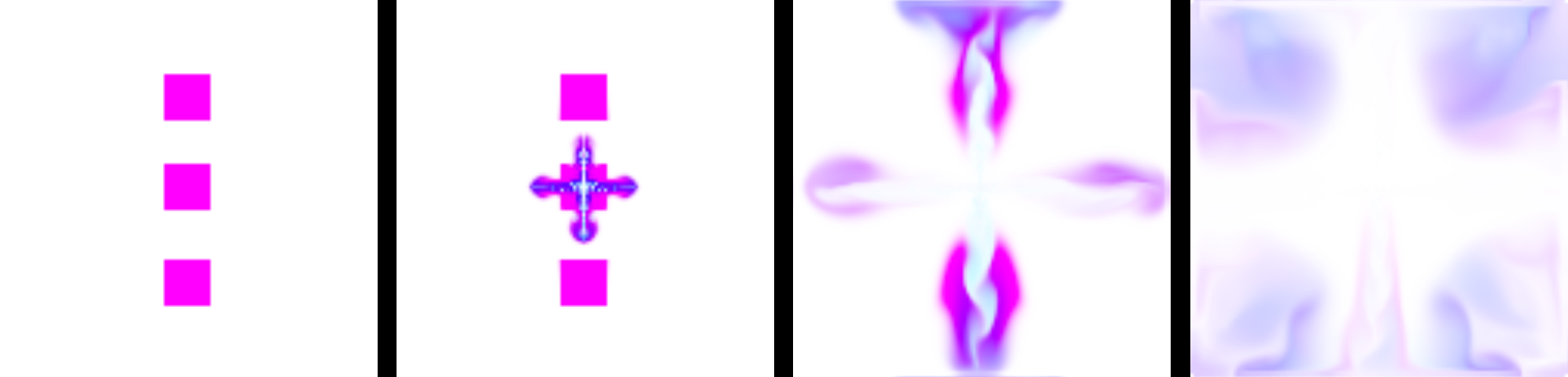
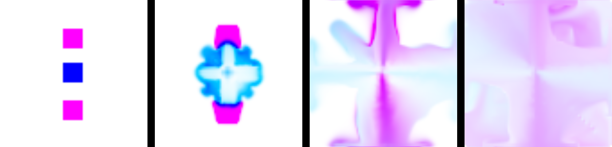
This example three-dimensional simulation demonstrating convection with a thin grid has initial conditions of three magenta squares in the top layer a long cyan rectangle in a lower layer (not rendered), and planar outward velocity sources in the middle magenta square. The second frame shows the cyan dye being pulled up into the top layer and mixing with the magenta dye. The third frame shows that eventually undyed milk is pulled up and pushed outwards.
Staggered Grid
Most computational fluid dynamics simulations use staggered grids introduced by the Marker-and-Cell method. In such a scheme, scalar fields in the fluid continue to be stored at grid cell centers, but the velocity field in the fluid is stored at grid cell faces (Griebel, et al. 1998). This staggering improves the accuracy of central differences for the velocity field projection calculation (Braley & Sandu 2010), at the cost of special handling for advection of scalar fields stored at grid cell centers along the velocity field stored at grid cell faces (Schlachter 2013). Note that the different components of fluid velocity are stored at different grid cell faces. This visualization of grid staggering in two dimensions translates easily to three dimensions:
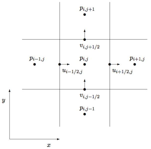
Scalar fields such as dye concentration $p$ are stored on cell centers in a grid indexed with $i$ and $j$ from 0 to the size of the grid $d_x$ and $d_y$ in the $x$- and $y$- dimensions, respectively. The corresponding $x$- and $y$- components of $\vec{u}$ are $u$ and $v$, respectively, and are stored on cell faces corresponding to their respective axes on a grid indexed with $i'$ and $j'$ from 0 to $d_x + 1$ and $d_y + 1$, respectively. Then $p_{i,j}$ associates with $u_{i',j'}$, $u_{i'+1,j'}$, $u_{i',j'+1}$, and $u_{i'+1,j'+1}$. (Schlachter 2013)
Staggering the grid slightly complicated the dye concentration’s semi-Lagrangian backtrace in that the velocities of the virtual particle for backtracing needed to be calculated by averaging the velocities at the faces of the grid. It also significantly complicated the handling of velocity boundary conditions.
Second-Order Backtrace
Stam’s method uses a Forward Euler step for the semi-Lagrangian backtrace from grid cell center $\vec{x}_G$ to backtraced position $\vec{x}_b$: $$\vec{x}_b = \vec{x}_G - dt * \vec{u}(\vec{x}_G)$$
This does not account for spatial variation of the velocity field $\vec{u}$, and a second-order method can improve backtrace accuracy. Schlachter uses the second-order Runge-Kutta (RK2) method, which first finds the velocity at a halfway backtrace: $$\vec{x}_m = \vec{x}_G - \frac{1}{2} * dt * \vec{u}(\vec{x}_G)$$ $$\vec{x}_b = \vec{x}_G - dt * \vec{u}(\vec{x}_m)$$ Note that $\vec{u}(\vec{x}_m)$ is calculated by trilinear interpolation on the grid for the velocity field $\vec{u}$. Implementation of this extension was straightforward.
Back and Forth Error Compensation and Correction
Kim, et al. demonstrated that the application of back and forth error compensation and correction (BFECC) to the advection step in Stam’s Stable Fluids method significantly reduces numerical dissipation and better preserves small-scale flow structures (Kim, et al. 2005). Following the review of Kim, et al.’s contribution by Costarelli, et al., let $\textbf{backtrace}(\vec{u}, \vec{\varphi}, dt)$ denote the backtrace step on a scalar or vector field $\vec{\varphi}$ along the velocity field $\vec{u}$ for time step $dt$. Without BFECC, advection of $\vec{\varphi}$ to the updated field $\vec{\varphi}_a$ is as follows: $$\vec{\varphi}_a = \textbf{backtrace}(\vec{u}, \vec{\varphi}, dt)$$ With BFECC, advection is as follows: $$\vec{\varphi}_b = \textbf{backtrace}(\vec{u}, \vec{\varphi}, dt)$$ $$\vec{\varphi}_c = \textbf{backtrace}(\vec{u}, \vec{\varphi}_b, -dt)$$ $$\vec{\varphi}_d = \vec{\varphi} + \frac{1}{2} (\vec{\varphi} - \vec{\varphi}_c)$$ $$\vec{\varphi}_a = \textbf{backtrace}(\vec{u}, \vec{\varphi}_d, dt)$$ This extension was easy to implement, though it significantly increased computational expense for improved accuracy:
This example simulation with a staggered grid, the RK2 backtrace, and the BFECC extension demonstrates better preservation of flows of different dyes, better spatial separation between dyes, and better preservation of fine shape features compared to Figure 2.
Parallelizing Computation
Performance profiling of the simulation with BFECC revealed that the performance bottleneck was in the backtracing step, specifically in the many trilinear interpolations performed by backtrace routine. To optimize the backtracing step, I used OpenMP to parallelize the simulation over the components of $\vec{\varphi}$ and the $i$ indices (indexing the columns) of the grid for $\vec{\varphi}$ in the backtrace step. This took two lines of preprocessor directives to implement and accelerated performance by a factor of 2. Further optimizations to relieve the bottleneck of trilinear interpolation would probably require porting my software to GPU code, such as is described in chapter 38 of GPU Gems (Harris 2004), to take advantage of linear interpolation at the hardware level. However, such further optimization was beyond the scope of my project.
Rendering Subsurface Scattering in Milk
Because milk has subsurface scattering, it is possible to see flows of dye beneath the surface of the milk. Thus, it was important that my simulation software approximate this effect. To achieve this, I sent the top several layers of the dye concentration grids to my fragment shader as a three-dimensional texture. I then developed the following heuristic approximation for subsurface scattering in a flat volume of milk with my fragment shader:
initialize CMYcolor as (0, 0, 0)
for each layer l from the deepest scattering layer to the surface layer:
    compute the depth of layer l in the 3-D texture's normalized coordinates
    compute blurredcolor as the result of applying a box blur on the l^2 texels in layer l neighboring the current fragment
    add blurredcolor to CMYcolor with a visibility multiplier
compute RGBcolor as (1, 1, 1) - CMYcolor
My implementation of the box blur for the above pseuedocode was inspired (with modifications) by TR Square Lab’s box blur algorithm (TR Square Lab 2015). I developed this heuristic approximation with inspiration from chapter 16 of GPU Gems (Green 2004), which describes methods for rendering subsurface scattering in complex three-dimensional objects.

This example simulation is identical to that in Figure 3, but with my subsurface scattering approximation in the fragment shader. This shader makes the layers look smoother and more realistic, and it is possible to see flows on different layers sliding past each other.
Interactive Usage
Finally, I developed an extensive keyboard-driven user interface to enable interactive use of the simulation software. In addition to keys for operating the camera from my initial reimplementation of Stam’s algorithm, I added keys to pause and unpause the simulation, adjust simulation timestep, and toggle grid boundary conditions on the top/bottom and left/right edges. I also added keys to adjust the CMY color channels, concentration, depth, and radius of circular dye droplets added by a left click with the mouse, and I added modifier keys to set the mode by which dye droplets would be placed on the grid - droplets could be placed by adding the concentrations to the grid, replacing existing concentrations on the grid, or as a constant source of dye on the grid. Similarly, I added keys to adjust the outwards flux, upwards flux, radius, and placement mode of circular soap droplets on the grid.
I implemented antialiased placement of circular droplets on the dye concentration grid with the following heuristic algorithm, which I developed independently by applying the concept of implicit functions introduced in the second lecture of CS 148:
for each grid index pair (i, j) of each cell in the bounding box of the circle centered at x and y with radius r:
    if i or j are out of bounds, continue to the next (i, j) pair
    compute dx and dy as i - x and j - y, respectively
    compute the outer distance as dx^2 + dy^2 - r^2
    if the outer distance is positive, continue to the next (i, j) pair
    initialize the antialiasing factor as 1
    if the outer distance is at least -2 * r:
        set the antialiasing factor to outer distance / (-2 * r)
        if dye concentration >= 1:
            divide the antialiasing factor by the concentration
        else:
            multiply the antialiasing factor by the concentration
    for each k from the index of the top grid layer to the full layer depth of the dye droplet:
        increase each color channel grid cell at (i, j, k) by the respective color channel value (C, M, or Y) * concentration * antialiasing factor
It is important to have some form of antialiasing because the simulation requires (for computational speed) grid sizes that are small enough such that individual grid cells are easily distinguishable:

Antialiased addition of dye droplets onto the dye concentration grid (right) greatly improves the visual appearance of the simulation (compare to left). Note that the fragment texture coordinate interpolation by OpenGL provides further smoothing of the edge of the dye droplet, producing the very smooth edge in the right image.
Final Results
With my software, I was able to run interactive fluid simulations. I used the apitrace tool with ffmpeg to record the OpenGL output of my program and export it to video, as documented by Adrian Scripca (Scripca 2014).
The following simulation of an 80-by-80-by-6 grid on a two-year-old Chromebook (Core i3) ran at a rate of 100 ms/frame, and demonstrates addition of dyes of varying color and radius and the visual appearance of subsurface scattering over time:
Below is a screenshot from a simulation run on a 128-by-72-by-8 grid:

Screenshot from a simulation
For comparison, here is a screenshot from Zoidis & Southgate’s video:

Screenshot from Zoidis & Southgate 2012
The qualitative similarity between these two screenshots in capturing the large-scale structure of these fluid flows demonstrates that my software is capable of approximating the essential visual aspects of dye advection in milk with soap droplets.
Below are recordings of simulations run on a 128-by-72-by-8 grid on a four-year-old quad-core laptop (Core i7). The simulations ran at a rate of 200 ms/frame:
Contributions and Acknowledgements
I did all the work related to this project. However, this project would not have been possible without helpful discussions with David Hyde, a teaching assistant for the course, or without the previously published work and additional resources cited throughout this report and listed below.
Similar Projects
As Stam’s Stable Fluids algorithm was first published in 1999, my review of prior work found numerous extensions of Stam’s algorithm in directions orthogonal to the direction my project took, including:
- Kristofer Schlachter’s fluid solver in C and OpenCL, which extended Stam’s 2-D fluid simulator to a staggered grid and used a RK2 backtrace, but focused on implementation of several other extensions for accuracy and performance. The paper accompanying Schlachter’s project, which I cite numerous times above, was very helpful for my project.
- Sven Olsen’s extension of Stam’s 2-D fluid simulator to handle solid obstacles.
- An unknown author’s extension of Stam’s 2-D fluid simulator to simulate smoke in three dimensions.
- Ingemar Rask and Johannes Schmid’s extension of Stam’s 2-D fluid simulator to simulate smoke and fire in three dimensions.
References
- Colin Braley and Adrian Sandu, “Fluid Simulation for Computer Graphics: A Tutorial in Grid Based and Particle Based Methods”. 2010. (pdf)
- Santiago D. Costarelli, Mario A. Storti, Rodrigo R. Paz, Lisandro D. Dalcin, and Sergio R. Idelsohn. “GPGPU Implementation of the BFECC Algorithm for Pure Advection Equations”. Cluster Computing, 17(2):243-254, June 2014. (url, pdf)
- Simon Green, “Real-Time Approximations to Subsurface Scattering”. GPU Gems, volume 1. Addison-Wesley, 2004. (url)
- Michael Griebel, Thomas Dornseifer, and Tilman Neunhoeffer, “Numerical Simulation in Fluid Dynamics”, Society for Industrial and Applied Mathematics. pp. 26-28, 1998. (url, pdf)
- Mark J. Harris, “Fast Fluid Dynamics Simulation on the GPU”. GPU Gems, volume 1. Addison-Wesley, 2004. (url)
- ByungMoon Kim, Yingjie Liu, Ignacio Llamas, and Jarek Rossignac. FlowFixer: Using BFECC for Fluid Simulation. In NPH ‘05 Proceedings of the First Eurographics Conference on Natural Phenomena, pages 51-56. 2005. (url, pdf)
- ByungMoon Kim, Yingjie Liu, Ignacio Llamas, and Jarek Rossignac. Advections with Significantly Reduced Dissipation and Diffusion. IEEE Transactions on Visualization and Computer Graphics, 13(1):135-144, January 2007. (url, pdf)
- Kristofer Schlachter, “Introduction to Fluid Simulation”. 2010. (url, pdf, slides)
- Adrian Scripca, “Capturing OpenGL Video on Linux”. Nov 2014. (url)
- Jos Stam. Stable Fluids. In Proceedings of the 26th Annual Conference on Computer Graphics and Interactive Techniques, SIGGRAPH ‘99, pages 121-128. New York, NY, USA, 1999. ACM Press/Addison-Wesley Publishing Co. (pdf, slides)
- Jos Stam. Real-Time Fluid Dynamics for Games. In Proceedings of the Game Developer Conference. March 2003. (url, pdf)
- TR Square Lab. A Simple Box Blur Implementation iN OpenGL/ES Using Shaders. Dec 2015. (url)
- Michael Zoidis and Jodie Southgate. Olafur Arnalds & Nils Frahm - a2 (Official Video). Erased Tapes Records. YouTube Video, November 2012. (url)